The following document is giving an overview of the basic knowledge
required to read properly the case studies / corrosion models files and submit (a) new file(s).
Metals have characteristic physical properties - they are good conductors of heat and electricity, are often lustrous, solid at room temperature (except Hg), ductile (can be worked without breaking), can be cast when in the liquid state, form positive ions in solution when they corrode, are cold and have a specific smell and sonority (particularly tin bronze with high tin content) (Selwyn 2004[1]).
The main ancient metals are gold (Au), silver (Ag), lead (Pb), copper (Cu), iron (Fe) and tin (Sn). More recent ones are zinc (Zn) and aluminium (Al). An alloy is a mixture of two or more elements in solid solution in which the major component is a metal. Alloys have, in most cases, been generated intentionally (to increase the hardness of the corresponding alloy, to lower its melting point, to improve its casting properties and make it cheaper). Trace elements contained in metals are very useful in archaeometry to date artefacts and reveal their provenance, but they can also change the physical properties of an alloy (for example arsenic (As) in Cu alloys and phosphorus (P) in Fe-carbon (C) alloys).
Relatively pure Au, Ag and Cu occur in nature in large amounts. Native Fe is very rare and can only be found in Greenland today (telluric iron). Most metal artefacts in human history have been extracted from ores (oxides, cuprite/Cu2O – hematite/Fe2O3 – cassiterite/SnO2 – alumina/Al2O3; carbonates, smithsonite/ZnCO3 – malachite/Cu2CuCO3(OH)2 and sulphides, galena/PbS – chalcopyrite/CuFeS2) by converting them through a reduction process at high temperatures (smelting). Unlike Cu, Pb, Ag, Au and Sn, the reduction of Fe arrived much later in human history. But advances in smelting technology and the abundant presence of iron ore has made Fe alloys the most widely used metal in human history (since the Iron Age, around 800 BC in Central Europe and the 3rd millennium in the Middle East). Aluminium cannot be produced by smelting. It requires the use of electrolytic processes and its industrial production parallels the development of electricity at the end of the 19th century (Selwyn 2004[1]).
The structure of metals is described in three levels. Firstly, on the atomic level, they are characterized by their metallic bonds. On the second level, metal atoms form crystals which show regular, repeated patterns in a three-dimensional arrangement called a lattice (most ancient metals develop either body-centred cubic (BCC) or face-centred cubic (FCC) lattices). Solid metals generally consist of many crystals clustered together to form a polycrystalline structure. The crystals are also known as grains in metallography, and the junctions between them called grain boundaries. These microstructures, the third level, can only be visualised after acid etching of the surface of the polished metal and observation with a metallographic microscope.
During the Neolithic period, when smelting first began, ores were only reduced in crucibles. Later they were reduced in furnaces. The reduction of copper and iron ores occurs in different ways. Iron smelting produces a spongy bloom which must be forged. Raw copper, on the other hand, was not forged, but melted to form artefacts. More recently (in Europe, from medieval times onwards) iron was obtained indirectly from the liquid state.
When solidifying in a mould, metal nuclei begin to form in the liquid solution of an impure metal or alloy. These nuclei grow as dendrites (tiny fernlike growths) which eventually meet each other. The faster the cooling rate, the smaller the dendrites. Dendritic microstructure is typical of cast ancient metal artefacts (Cu-Sn alloys or so called Sn bronzes, arsenical Cu, Ag-Cu alloys, etc.). In binary alloys such as Sn bronze, the cores of the dendrites are rich in Cu while their outer regions are Sn-rich (this element having a lower melting point). This phenomenon is known as dendritic segregation. When purer liquid metal is cooled more slowly, dendrites may not form at all. Instead an equiaxial, hexagonal grain structure develops. Such a structure can also be obtained by annealing, i.e. extended exposure to high temperature of the original dendritic structure (Scott, 1991[2]).
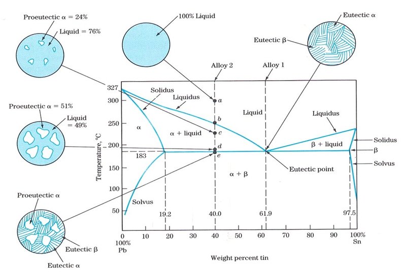
Fig. 1: Phase diagram of Pb-Sn alloys with sketches of the microstructure observed depending on the composition of the alloy (from http://www.benbest.com/cryonics/lessons.html, accessed on January, 02 2018). The eutectic point corresponds to a mixture of elements having a unique chemical composition that solidifies at a lower temperature than any combination of the same constituent elements.
Phase or equilibrium diagrams (plots of temperature against the relative concentrations of two components in a binary alloy, Fig. 1) are used by metallurgists to predict what phases should be present in an alloy at equilibrium (very slow cooling rate) and to interpret the microstructure of metal alloys observed under a metallographic microscope. In simple cases (such as Pb-Sn alloys – Fig. 1), the microstructures are indications of the composition of the alloy as well as the different phase transformations from molten metal. In the example given, Sn is more soluble in Pb than vice versa. As molten Sn and Pb mixtures cool, they solidify into combinations of two solid phases, labelled in the diagram as β (rich in Sn) and α (rich in Pb). The carbon (C) content in steels can be determined through metallographic studies with the help of the Fe-C diagram (see next section).
Except for cast objects (such as sculptures, tools, and ingot), most metal artefacts are additionally cold or hot worked to obtain specific shapes. Annealing is required to release stress within the metal. But this exposure to sometimes high temperature (100-1200°C, depending on the metals) modifies the microstructure of the material, though not the inclusions, which remain elongated and deformed. FCC metals (Cu, Al, Ag, Pb) can be cold worked and annealed repeatedly (the combination of both processes is referred to as hot-working). As a consequence twins appear within the grains. Tempering (exposure to temperatures between 100 and 600°C) of steel is sometimes carried out instead of annealing (500-800°C). Final cold working is revealed on cross-sections by slip (or strain) lines.
The understanding of metal microstructures and the effect of mechanical and heat treatments on the microstructures of metal artefacts dates from the end of the 19th century, when metallographic microscopes and phase diagrams were first developed.
Copper is one of the earliest metals to be used by humans (8500 BC, northern Iraq: Selwyn 2004[1]). Copper alloys are often divided in four large families: pure Cu, bronzes (Cu/Sn), brasses (Cu/Zn) and quaternary alloys (Cu/Sn/Zn/Pb). The oldest Cu alloys contained As or Sb. Zn, Pb or As are often secondary elements in bronzes whereas brasses can contain Sn or Pb. Cu/Ni, Cu/Zn/Ni and Cu/Al alloys have been developed in recent times (19th century).
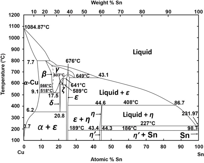
Fig. 2: Phase diagram for Cu and Sn (from https://www.researchgate.net/figure/Figure-27-The-Cu-Sn-phase-diagram-This-phase-diagram-will-be-very-relevant-for-the-rest-of-this_316317422_fig16, accessed on January, 02, 2018).
As cast, bronzes are categorized as belonging to the Cu α phase only if their Sn content does not exceed 4 mass% (Fig. 2). Above this value the alloys have an α (alpha) + δ (delta) microstructure. Depending on the Sn and secondary elements (Pb, As) content, as well as the heat treatments applied, bronzes are either constituted of Cu α phase or Cu α phase associated to the eutectoid α + δ phase. Pb (up to 7 mass% in the alloys studied) is insoluble in copper alloys and forms inclusions. Their fineness and regular distribution give high quality alloys.
Ancient copper alloys are more porous than modern ones and contain Cu2S as well as heavy metal (Pb-rich) inclusions, whereas modern copper alloys (from the 17th century onwards) contain Cu2O inclusions.
Typically, pure annealed copper shows a hardness of HV1 40-50. Small additions of Sn or Sb increase this slightly, to HV1 70-100. Cast tin bronzes or alloys with final cold working show the highest hardness values (HV1 between 120 and 180).
Iron produced by smelting appears around 1300-1200 BC in the Mediterranean region (Selwyn 2004[1]) and prior to 4000BC in the Near East. Iron alloys can be divided in three large families: iron, steel and cast iron. The main difference between them is their carbon (C) content. Carbon lowers the melting point of Fe by several hundred degrees and increases its hardness. Fe (α phase, ferrite, see Fig. 3) has a concentration of C lower than 0.02 mass%), steel contains higher amounts of C (up to 2 mass%) whereas cast iron has a C content usually between 2 and 4 mass%. Sub-families exist for steels: hypo-eutectoid or hyper-eutectoid (C content below or above 0.8 mass% resp.) and cast irons: in grey cast iron free C occurs as flakes of graphite (not represented in Fig. 3) while in white cast iron all the C is taken up as cementite (Fe3C), pearlite (mixture of ferrite and Fe3C) and ledeburite. Iron and steel produced by direct reduction have coexisted since the end of the Medieval times (12-13th centuries). Later the process of indirect reduction became more and more important. In the indirect reduction a blast furnace is first used to produce pig iron (containing up to 3.5–4.5% C), then in a second step the metal is refined to reduce the content in carbon and other elements, transforming the cast iron to steel. A high P content (up to 2 mass%) in cast iron favours the growth of interconnected networks of steadite (Fe3P). Specific iron alloys were developed in the 19th century such as Thomas ferritic steel containing up to 0.2 mass% Mn as well as carbonitrides.
Fig. 3: Partial phase diagram for Fe and C to form the metastable Fe3C (cementite) at the 6.67 mass% C end of the diagram (from http://sv.rkriz.net/classes/MSE2094_NoteBook/96ClassProj/examples/kimcon.html, accessed on January, 02, 2018). The bottom scale of the diagram is mass% C.
Ancient wrought iron contains many slag inclusions originating from slag included during bloomery smelting and not expelled by primary smithing (refining a bloom). Most slag inclusions in iron produced by the bloomery process or by smithing are composed of wustite/FeO dendrites and fayalite/Fe2SiO4 in a glassy matrix. On the other hand recent iron contains only tiny FeO inclusions and sometimes none at all. The presence of P (up to 0.3-0.45 mass%) in iron increases its hardness and creates Neumann bands within the grains if the metal has been cold worked. Thomas steel contains MnS inclusions.
In the past, smiths knew how to modify the properties of iron bars. They could reinforce them by soldering several bands, hardening them locally on the surface through C enrichment. By quenching steel they could considerably increase its hardness (through the formation of martensite) but this increased its fragility too. Such steel artefacts were useless and had to be tempered, allowing the material to retain some of its hardness while being partly re-homogenised.
Typically wrought iron has a hardness in the range HV1 90-110. Hypoeutectoid to eutectoid steels and grey cast iron have hardnesses around HV1 120-200, depending on their C content. White cast iron is much harder. After cold working, or as a result of alloying with P or As (higher than 0.1 mass%), the HV1 can increase to 185-200. The average hardness of quench-hardened eutectoid steel is about HV1 690. After tempering, the HV1 of bainite decreases to 350-360.
While Zn is commonly found as a constituent of copper alloys, its industrial production only began in 1738 due to difficulties in collecting the metal (which evaporates at 907°C) during the reduction of calamine (ZnCO3) (Selwyn 2004[1]). Specific alloys (Zamak-Zn/Al/Mg/Cu) were developed later in response to specific needs.
Aluminium alloys were developed in the later part of the 19th century. Pure aluminium was first produced chemically at a very high cost. When electrolytic production was developed in 1886 the metal became cheap and very quickly found use as an important industrial material. Since 1970, aluminium alloys are divided in families: Al, Al/Cu, Al/Mn, Al/Si, Al/Mg, Al/Mg/Si, Al/Zn. Some of them are cast, others are wrought alloys hardened by heat treatment (heat-treatable: Al/Cu, Al/Mg/Si and Al/Zn) or by the presence of the alloying elements (non-heat-treatable: Al, Al/Mn, Al/Mg) (Selwyn 2004[1]).
Fig. 4 shows that during the cooling of an alloy containing 4.6 mass% Cu, Cu separates from Al (Al contains less than 0.5 mass% Cu at room temperature) to form the intermetallic compound CuAl2 (which corresponds to the θ phase in the phase diagram).
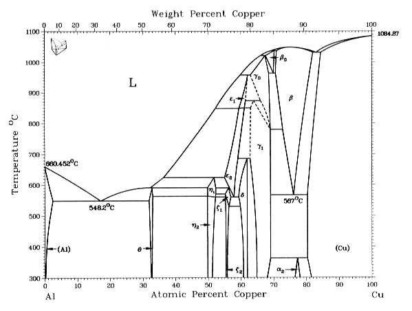
Fig. 4: Phase diagram for Al and Cu (from http://chemsoc.velp.info/alloys.php, accessed on April,
06, 2015).
Most metal artefacts (except pure gold) undergo corrosion, an electrochemical process which transforms the thermodynamically unstable metal artefact back to its thermodynamically stable mineral structure. There are two ways to slow down this natural process, either through preventive conservation strategies or interventive conservation (Fig. 5).
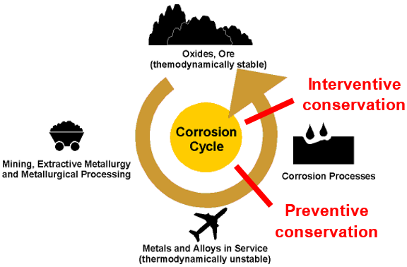
Fig. 5: The thermodynamic corrosion cycle (from https://www.nitty-gritty.it/corrosion-process/?lang=en, accessed on January, 02, 2018).
The study of corrosion layers not only contributes to the understanding of the corrosion mechanisms, but it can help to locate the limit of the original surface. For slightly corroded artefacts exposed to the atmosphere, the original surface is often visible. For buried artefacts, the original surface is considered to be the surface of the metal artefact when it was abandoned (Bertholon 2000[3]). This might be obscured by corrosion products, but markers within the corrosion crust can help localising it. For instance SiO2 particles are external markers and can only be brought into the corrosion crust by the surrounding environments. Unlike Cu, Sn is not a mobile ion that can move to the surface of Sn bronzes (Cu-Sn alloys) to form oxides during corrosion. It is therefore considered as an internal marker. Corresponding markers of the original surface, such as inlays, tool marks, natural separation of corrosion layers and a more densely packed corrosion, can all indicate that the limit of the original surface has been reached. When corresponding markers are absent, elementary analysis of metallographic samples can help to define the limit of the original surface (presence/absence of Sn in a corroded bronze, location of Si, etc.).
Often the colour and physical appearance of corrosion products on metal artefacts are used to suggest the family of metal in which the artefact is made.
Corrosion usually starts locally, through a pit. Pitting corrosion is a galvanic phenomenon during which the metal is consumed. It can develop extensively only on recent metal alloys (aluminium alloys, stainless steel). On ancient and historic metal artefacts, corrosion moves from local to general. The thickness of the corrosion crust depends on the material (thinner for copper alloys than iron alloys), the exposure or burial conditions and time. The remaining metal can be in good condition or partially mineralized due to intergranular or transgranular corrosion. Specific forms of corrosion (stress corrosion cracking, fatigue) develop on metals exposed to mechanical stress such as components from technical or horological objects.
All ancient and historic metals have, during use, been exposed to the atmosphere, thereby suffering from atmospheric corrosion. Relative humidity and temperature are the main parameters governing atmospheric corrosion, but some pollutants can increase it dramatically. Chlorides, which induce the active corrosion of copper and iron based alloys, are typical outdoor pollutants. Acetic acid vapour produced by freshly cut oak is a typical indoor pollutant that affects lead and zinc (Selwyn 2004[1]). In slightly polluted atmospheres, metal artefacts become covered with time by a thin, dense, protective, natural patina which may be aesthetically pleasant (green copper-sulphate CuSO4,3Cu(OH)2 brochantite on copper roofs) (Selwyn 2004[1]).
The naturally formed patina on historic copper alloy artefacts (such as outdoor Sn bronzes) has been studied extensively by conservation professionals who wish to know whether the corrosion is active or passive. For outdoor bronzes, the main process of Cu-Sn corrosion is the selective dissolution of Cu (Robbiola and Hurtel 1991[4]). Sn oxidation occurs first, forming insoluble compounds in the corrosion layer. Then the Cu oxidises and, depending on the conditions of exposure, forms a protective layer (referred to as type 1 patina) or a non-protective layer (referred to as type 2 corrosion) as shown in Fig. 6. The limit of the original surface can only be determined in type 1 patina.
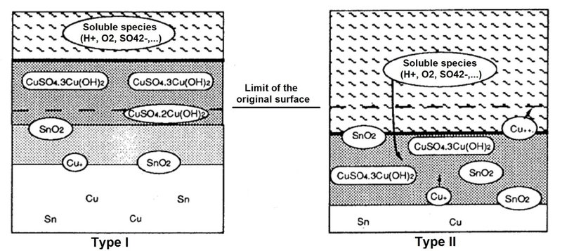
Fig. 6: Schematic representation of corrosion types in outdoor bronze (from Robbiola & Hurtel 1991).
Atmospheric corrosion of historic iron has only recently been studied by Monnier (Monnier 2008[5]). Due to instrumental limitations it has been very difficult to study the complexity of iron corrosion products formed in uncontrolled atmospheres. The corrosion crust was thought to consist of an inner dense goethite/αFeOOH layer and an outer porous and cracked lepidocrocite/γFeOOH layer. Using microscopic analytical techniques such as mXray diffraction or mRaman spectroscopy, Monnier showed that the marbling effect observed in the corrosion crust in cross-sections was due to goethite and iron (III) oxyhydroxide (ferrihydrite) phases connected or not to the remaining metal. As shown in Fig. 7, lepidocrocite can be found locally as well as akaganeite/βFeOOH. Magnetite/Fe3O4 is not a typical corrosion product. Often the limit of the original surface is difficult to determine within the corrosion crust of iron based artefacts.
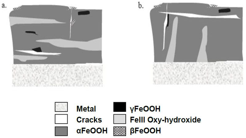
Fig. 7: Schematic distribution of iron compounds in the corrosion crust of an iron artefact exposed outdoors. Marbling not connected (a) or connected to the metal (b). From Monnier 2008.
In clean air (i.e. no pollutants or salts) almost no corrosion develops on pure aluminium and its alloys due to the presence of a thin (about 25Å) protective film of aluminium oxide. In the presence of contaminants, however, the corrosion layer thickens, dulling the metal surface. The corrosion rate is strongly increased by the presence of chlorides, and pitting corrosion develops further. Depending on the nature of the alloy pitting may expand through the entire metal thickness or develop as intergranular corrosion or / and exfoliation (Selwyn 2004[1]). Often the limit of the original surface is preserved on aluminium alloys.
In clean air, zinc alloys normally oxidise to form stable ZnCO3 (Selwyn 2004[1]). Zn-Al alloys often suffer from intergranular corrosion. When this happens the alloys lose strength, start to crack and eventually disintegrate (Selwyn 2004[1]).
Metal artefacts will only survive if they are buried in soil after being abandoned. The corrosion processes which occur depend on the type of soil (its chemistry in terms of composition, granulometry, resistivity, etc.), the underlying geology, the depth of burial, the natural salt loading of the soil, the presence of external pollutants, the water-retentive capacity of the soil, its oxygenation and the local hydrological regime. In marshy, flooded or submerged sites, anaerobic corrosion may develop in the presence of sulphato-reducing bacteria. If this occurs, the corrosion products are rich in sulphur (Selwyn 2004[1]).
The general corrosivity of an aqueous medium can be given by Eh (oxidation-reduction potential in soil)-pH diagrams such as the one given in Fig. 8. The two dashed diagonals delimit the range of stability of the aqueous medium. Just below the upper limit we find an aerated media. As the potential Eh decreases the medium becomes depleted of oxygen. Anaerobic conditions are found just above the lower limit of the aqueous medium stability (Garrels and Christ 1965[6]).
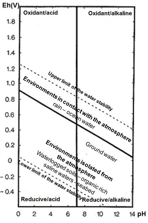
Fig. 8: Stability limits in soils for natural waters in terms of Eh and pH at 25oC (from Garrels and Christ 1965).
Pourbaix diagrams combine the information given in Fig. 8 with the general behaviour of pure metals (immunity, corrosion, passivation) in pure water. This thermodynamic approach can help to predict the behaviour of a metal in a specific environment (within the field of stability of the aqueous medium). For instance Fig. 9a shows that when the pH lies between 8 and 12, Cu passivates (forming Cu(OH)2 and cuprite/Cu2O) while in acid media it corrodes to Cu2+. When the concentration of CO2 in the medium increases, malachite/CuCO3Cu(OH)2 and azurite/2CuCO3Cu(OH)2 may develop in addition to cuprite in slightly acidic and oxidising conditions, while a tenorite/CuO / cuprite mixture will form in alkaline conditions (Fig. 9b). If the medium contains S (anaerobic conditions), Fig. 9c shows that covellite/CuS, chalcopyrite/CuFeS2 or chalcocite/Cu2S will form. Predictions become less certain, however, when alloys containing several elements are considered, since several Pourbaix diagrams must be used in parallel.
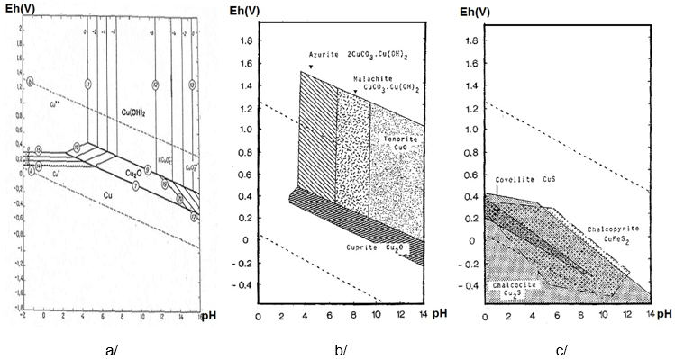
Fig. 9: Pourbaix diagram of Cu in H2O at 25°C (Pourbaix 1963[7]) and simplified Pourbaix diagrams of the system Cu-CO2-H2O and Cu-S-H2O (Pourbaix 1977[8]).
Over the years buried copper alloy artefacts develop either a type 1 patina or a type 2 corrosion crust. Compared to artefacts exposed to atmospheric attack, the main difference is that the corrosion is usually much more significant. Chlorides concentrate at the metal - corrosion crust interface and are often at the origin of a type 2 corrosion (Robbiola 1990[9]). A particular kind of corrosion develops in lake sediments and has been thoroughly studied by Schweizer while investigating objects from the site of Hauterive-Champréveyres NE on the shores of Lake Neuchatel (Schweizer 1994[10]). Of those objects, 70% were covered by a smooth, dense, brown patina, referred to as lake sediment patina (type I patina). The remaining artefacts have either developed a thick terrestrial blue-green corrosion layer, or a mixture of terrestrial corrosion crust and lake sediment patina (both are type 2 corrosion). The objects were found either in sandy soil or organic-rich soils which correspond to human occupation levels (pH between 7.1 and 7.7). Neither the composition (bronzes with a Sn content ranging between 5.5 and 9.5 mass% and minor contents of As, Ni, Pb and Sb not added intentionally) nor microstructure have any effect on the corrosion type. Lake sediment patina mainly consists of chalcopyrite/CuFeS2 while the terrestrial corrosion crust is a mixture of malachite/CuCO3Cu(OH)2, antlerite/CuSO4(OH)4 and posnjakite/CuSO4(OH)6H2O. To form chalcopyrite the bronze corrodes first by the traditional dissolution of Cu and an enrichment in Sn. Cu is redeposited afterwards as chalcopyrite in a deaerated S- and Fe-rich environment. The limit of the original surface of the object can be located between the chalcopyrite and the Cu depleted but Sn-rich inner corrosion layer. The lake sediment patina corresponds to artefacts that remained buried in anaerobic conditions while the terrestrial corrosion crust / lake sediment patina mixture is due to a change in the burial conditions from anaerobic to aerobic (with partial dehydration) (Schweizer 1994[10]).
Iron based artefacts buried in soil are covered with a thick corrosion crust that consists of an inner Dense Product Layer (DPL, in contact with the metal) that can contain the limit of the original surface, and a more porous layer called Transformed Medium (TM) followed by soil (Fig. 10).
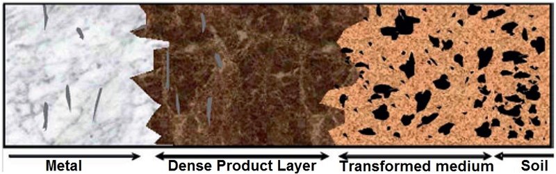
Fig. 10: Diagram of a transverse section through an iron archaeological artefact (from Saheb and al. 2007[11]).
In aerated soil that contains only low concentrations of carbonates, sulphates, phosphates and chlorides, the DPL mainly consists of goethite/αFeOOH with marbling of magnetite/Fe3O4 and maghemite (or Fe(III) oxyhydroxides). In most cases this marbling is not connected to the metal substrate. The DPL contains large cracks often filled with CaCO3 (Fig. 11a). When the soil contains chlorides, akaganeite/βFeOOH may form after excavation as the object dehydrates and oxygen gains access to the metal core where chlorides concentrate. In deaerated soil that contains carbonates, FeCO3/siderite is observed adjacent to the metal surface as well as iron sulphides resulting from the action of sulphato-reducing bacteria (Fig. 11b) (Dillmann 2004[12]).
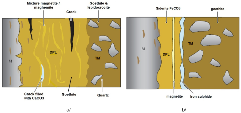
Fig. 11: Schematic representation of corrosion crusts on iron based artefacts buried in aerated (a) and deaerated (b) soils (from Dillmann 2004).
To build the corrosion models, an examination protocol
has been defined as follows: the remaining metal and corrosion crust of all
samples are first studied by metallography under an optical microscope. Since
metallography is based on known alloys, the chemical composition of all metals
under consideration has to be determined.
Metallography
is based on the study of metal samples polished to a mirror finish or
cross-sections of metal samples embedded in a synthetic resin. The examination
is carried out under an optical microscope (inverted in the present case, Fig. 12) in reflective mode, the metal having first been given a mirror-finish
(bright field examination). The morphology of the samples (i.e. the remaining
metal, inclusions, cracks, form of corrosion and corrosion layers) is studied
under these conditions. The observation starts at low magnification (x12.5) and
if necessary is continued to x1000. Metals appear white (Fe alloys) or pink (Cu
alloys) in bright field illumination, whereas most of the corrosion products
and non-metallic inclusions appear in various shades of grey. Observation under
polarised light allows the different layers within the corrosion crust to be
distinguished by their colour. This is only possible, however, for
magnifications between x50 and x200.
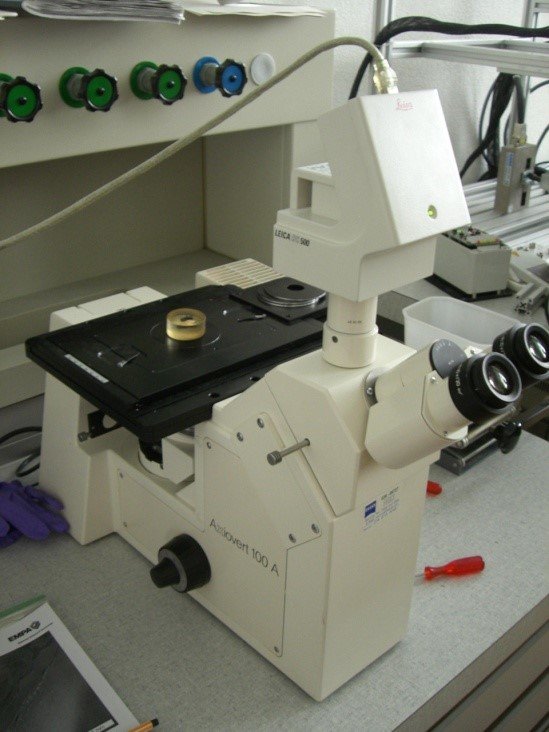
Fig. 12: Inverted reflective light microscope used for metallographic investigation, Empa. The sample is positioned upside down on the platform of the microscope.
After etching, the microstructure of the metal surface is revealed. This part of the examination is known as microscopic study. Etching causes a chemical reaction with the metal resulting in a selective attack or corrosion. Most reagents reveal grain boundaries and twins after a brief application with a cotton swab (a few seconds to some tenths of seconds). Oberhoffer’s reagent, used on Fe alloys, reveals segregations and requires a total immersion of between 10 and 30 seconds.
Hardness testing of the metal is the last step of the metallographic investigation. The aim is to better understand and interpret the manufacturing techniques used to produce the metal and the influence of the alloying elements. For this purpose Vickers hardness testing is used. A small pyramidal diamond indenter is forced into the surface of the specimen with a predetermined force. The resulting impression is observed and measured under the microscope; this measurement is then converted into a hardness number. Vickers hardness numbers are designated by HV plus the load (HV1 means Vickers hardness testing with a load of 1 kp or 9.8Newton). For this study each measurement is repeated three times and a mean value is calculated. The resulting hardness values can be compared to certain references (Scott 1991, p82[13]) for all the alloys studied here except those of Zn.
Grinding for the metallurgical examination begins with wet SiC papers ranging in fineness from 2000 to 4000 microns/grit for Cu, Al, Mg and Zn alloys and with 1000 microns/grit for Fe alloys. Subsequent polishing is performed with monocrystalline diamond paste starting with 6 microns grade and for most of the metals finishes with 1 micron. Very soft metals, such as Al, Mg and Zn alloys, are given a final polishing with Eposil F with a grain size of 0.1 micron.
Reagents are specific to the relevant metal alloys.
- Reagents for Fe alloys
Most of the Fe-based samples are first etched with Oberhoffer’s reagent, which has the following composition (Schumann 1991, 737[14]):
30g FeCl3
1.0g CuCl2
0.5g SnCl2
50mL hydrochloric acid
500mL ethanol
500mL distilled water
Oberhoffer’s reagent is a macroscopic reagent which renders visible phosphorus (P) segregations. It is not frequently used in modern metallurgical research, but common in the archaeometallurgical context. P-rich areas are not attacked by this reagent, whereas those free of segregations become dark coloured or brown because of Cu deposition on the surface. Since P is an element which diffuses only slowly into Fe, it often forms segregations after deformation and recrystallization (Schumann 1991, 115, 372, 406). The effect of Oberhoffer’s reagent on Fe alloys has been used specifically with the aim of studying archaeomaterials (Stewart et al. 2000a[15]). For this purpose modern iron and steels (C 0.02, 0.7, 0.95 mass%) containing P (0.4, 2.4 mass%), Ni (1.1, 1.3 mass%) and As (0.24 mass%) were etched since all three elements are important in ancient and historic Fe-C alloys. The authors showed that this reagent also reacts with steel components, particularly cementite (in pearlite and on grain boundaries which are also free of Cu deposition). Therefore, P segregation in cementite bearing steel is difficult to detect. The study also showed, however, that Ni and As are affected by the etching. In P-bearing iron, Oberhoffer’s reagent can differentiate P contents in samples of less than 0.05 mass%. Individual segregations of approximately 0.2 mass% As, 1 mass% Ni and 0.1 mass% P in a Fe-α-matrix will appear bright after etching due to extreme delay of Cu deposition.
The same samples are ground and polished again before nital etching. Nital has the following composition, after Schumann 1991, 737:
1-5mL nitric acid
100mL ethanol
Nital is used to make visible the grain structure of Fe-C alloys. The reagent affects grain boundaries and cementite constituents (Fe3C), which become darker than the rest of the structure. It also makes ghost structures visible. Ghost structures, which occur in P-rich iron, mark sharp changes in local P content in the solid solution. The degree of attack depends upon the local P content (Stewart et al. 2000b[16]).
- Reagent for Cu alloys
Of the large number of reagents available for use with copper alloys, only one is chosen to etch all the copper alloy samples. This is a ferric chloride reagent with the following composition:
8g FeCl3
120mL distilled water
20mL hydrochloric acid
240mL ethanol
Scott gives a large variety of compositions for this reagent (Scott 1991, 72[13]). It reveals grain contrast, twins and dendrites.
- Reagent for aluminium alloys
All aluminium samples are nital etched. Good results are obtained for nearly pure aluminium showing the grain structure, but the reagent dissolves the Sn-rich phase in the as-cast AlCuSnZn alloy.
After etching, the metal microstructure is documented with digital photography combined with the inverted light microscope. Among the documented data is the determination of the grain size, which is related to annealing times and temperature. Large grains are formed after a long period of annealing or exposure to high temperatures. Small grains occur after a short period of annealing or in alloys that have been heavily cold worked. For Cu alloys the grain size is either measured directly (with the help of an eyepiece lens with a graduated scale), or from the photograph (with the help of the program ImageAccess). In the case of Fe-C alloys, chart rating according to ASTM norms (today E112 is in use) is carried out. For ancient objects the charts from DIN50-601 (which is no longer used in modern metallography) are very helpful, with charts for austenite, ferrite and deformed ferrite available, varying from ASTM no.1 to 10. To determine the grain size, a magnification of x50, x100 or x200 can be chosen to compare a circular image area with the charts, thus allowing the ASTM number to be estimated.
As mentioned before, metallography is based on a known chemical composition of metallic samples. The following techniques used on the samples are detailed below:
- Laser ablation combined with inductively coupled plasma mass spectroscopy (LA-ICP-MS),
- Electron micro probe analyzer combined with wavelength dispersive X-ray spectroscopy (EPMA/WDS),
- Inductively coupled plasma optical emission spectrometry (ICP-OES),
- Scanning electron microscope combined with energy dispersive X-ray spectroscopy (SEM/EDS).
Except SEM/EDS, all the other techniques are useful in detecting trace elements, because they have low detection limits: for EPMA/WDX and ICP-OES the limit is in the best case 0.01 mass%, whereas for LA-ICP-MS this reaches 1 mg/kg in the best case (0.0001 mass%). SEM/EDS is a semi-quantitative analytical method because no calibration is carried out - the detection limit is around 0.5 mass%.
LA-ICP-MS analysis is based on the ablation of the surface of the sample with a laser to form a crater. The very fine ablated material is transported by a flow of gas (argon or helium) into the plasma of the ICP-MS. In the hot plasma the material is initially atomized then ionized. The various ions have different masses which are detected by the spectrometer and counted. LA-ICP-MS analysis on Fe-C alloys is carried out after metallographic examination. Since nital reagent has no influence on the chemical analyses of the metal, no grinding and polishing is necessary. This is, however, not true for Cu alloys where the reagent contains Fe and Cl, elements that would falsify the chemical analysis. Cu alloy samples therefore have to be ground and polished again before carrying out LA-ICP-MS.
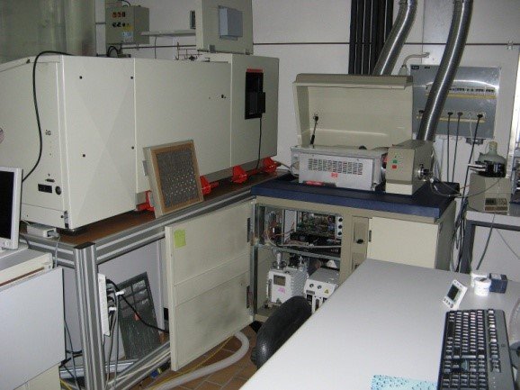
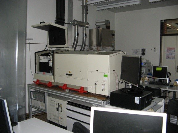
Fig. 13: LA-ICP-MS: the ICP-MS at the back with the back side of the laser on the left (a/) and the front side of the laser (b/), Laboratory of Analytical Chemistry, Empa.
At Empa, the application of LA-ICP-MS to ancient and
historic Fe alloys is developed according to settings devised by Devos (Devos
et al. 2000, Fig. 13[17]).
In the past, only V, Cr, Mn, P, Co, Ni, Cu and As were analysed. The
calibration is carried out by measuring two standard materials (NIST 1262 and
ARL 1721) whose elemental composition is known. Today, for quality control
purposes, a standard material is analysed during each measurement campaign
(NIST 1162). The following elements have also been added to the existing list
of analysed elements: Al, Ti, Mo, Ag, Sn, Sb and W. The same settings are
applied to analyse the other Fe alloy samples at the ETH. The detection limits
for most elements are under 10 mg/kg, except for P which is below 100mg/kg. On
the etched samples the areas to be analysed are marked with a diamond cone
under the optical microscope. The reason for this marking is to avoid
non-metallic inclusions (slag, corrosion) and segregations, especially along
welding seams. Since ancient and historic alloys have a heterogeneous chemical
composition, several analyses (3 to 5) are carried out for each sample. From
these results a median value is calculated (rather than a mean, so as to give
less weight to results which are very different). To give some idea of the
heterogeneity of the elements in the alloy, the relative standard deviation
(RSD) is also given. At the University of Warsaw the standard materials NIST
454, BAM 211, BAM 227 and BAM 374 have been used to calibrate the copper alloy
samples. Calculation is done in a different way than for the iron, making it
impossible to determine fixed values for the detection limits. The analysed
elements are P, Fe, Co, Ni, Zn, As, Ag, Sn, Sb, Pb, Bi and S. The remaining
metal is assumed to be copper.
Table 1 gives the specific settings used by the three laboratories that applied LA-ICP-MS on the samples.
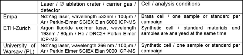
Table 1: Conditions of use and settings of LA-ICP-MS instrumentation.
An electron microprobe (EMP, also known as an electron probe micro-analyser, EPMA or electron micro probe analyser, EMPA) is a type of electron microscope that uses a beam of electrons to illuminate the sample and produce a magnified image. Electron microscopes (EM) have a greater resolving power than optical microscopes, because electrons have wavelengths about 100,000 times shorter than visible light, allowing them to achieve a 50pm resolution and magnifications of up to about 10,000,000x. Ordinary, non-confocal optical microscopes are limited by diffraction to about 200nm resolution and useful magnifications below 2000x.
The electron beam has various effects on the sample: it produces characteristic X-ray radiation, secondary electrons and backscattered electrons. The characteristic X-rays are used for chemical analysis. Specific X-ray wavelengths are selected and counted, either by wavelength dispersive X-ray spectroscopy (WDS) or energy dispersive X-ray spectroscopy (EDS). WDS utilizes Bragg diffraction from crystals to select X-ray wavelengths of interest and direct them to gas-flow or sealed proportional detectors. In contrast, EDS uses a solid state semiconductor detector to accumulate X-rays of all wavelengths produced from the sample. While EDS yields more information and typically requires a much shorter counting time, WDS is a more precise technique due to its better X-ray peak resolution[18]. All elements from boron (B) upwards can be analysed. Chemical composition is determined by comparing the intensities of characteristic X-rays from the sample material with intensities from test samples of known composition (standards).
For the EPMA/WDS analyses carried out at the Department of Materials, University of Oxford, the settings employed are described in Northover 1998[19], and older publications[20]: “Operating conditions are accelerating voltage 25kV, a beam current of 30nA and a take-off angle of 62°. Thirteen elements are analysed; pure element and mineral standards are used for calibration (counting time of 10 s per element). Detection limits are mainly 100 and 200 mg/kg, with the exception of 300mg/kg for Au and 0.2 mass% for As. The latter is due to the well-known interference between the principal lines in the Pb and As spectra, the Pb L-alpha- and the As K-alpha-line. The relatively strongly Pb M-alpha-line can be used, but for As the weak K-beta-line is required, hence the degradation in performance. Another small source of inaccuracy is the analysis of Pb. The correction software assumes that Pb is in solid solution in the bronze whereas in fact it can be present as large discrete particles. Three areas, each 30 x 50µm, are analysed on each sample; the mean compositions for each sample, normalised to 100%, are presented in the tables. All compositions are in mass%.”
Inductively coupled plasma atomic emission spectroscopy (ICP-AES), also referred to as inductively coupled plasma optical emission spectrometry (ICP-OES), is an analytical technique used for the detection of trace elements. In this study an ICP-OES coupled with argon plasma is used. In this type of emission spectroscopy the inductively coupled plasma produces excited atoms and ions that emit electromagnetic radiation at wavelengths characteristic of a particular element. The intensity of this emission is indicative of the concentration of the element within the sample[21].
Destructive samples (25 to 40mg) are drilled from the metallic parts of Cu alloys (Kläntschi 1995, 14-15[22]). They are then dissolved in a mixture of hydrochloric and nitric acids. The solution obtained is pumped to a nebulizer where it is converted into a mist and introduced into the plasma flame. The sample material immediately collides with the electrons and charged ions in the plasma and is broken down into charged ions. The various molecules disintegrate into their respective atoms which then lose electrons and recombine repeatedly in the plasma, giving off radiation at the characteristic wavelengths of the elements involved. The intensity of each line is then compared to previously measured intensities of known concentrations of the elements, and their concentrations are computed by interpolation along the calibration lines. Eleven elements are detected (Cu, Sn, Pb, As, Sb, Ag, Ni, Bi, Co, Zn, Fe). For quality control two reference materials with a known composition are regularly analysed (BAM 211 and 227). The detection limit varies between 20 to 500mg/kg for the chosen elements.
The SEM/EDS functions in a similar way to EPMA/WDS. When the electron beam used to illuminate the sample interacts with the specimen, it loses energy by a variety of mechanisms. The lost energy is converted into alternative forms, such as the emission of low-energy secondary electrons (SE-mode) and high-energy backscattered electrons (BSE-mode), or X-ray emission. These emissions sources carry information on the properties of the specimen surface, such as its topography (SE-mode) and chemical composition (BSE-mode and X-rays). Because the SEM imaging technique relies on surface processes, it is able to image bulk samples up to many centimetres in size and (depending on instrument design and settings) has a great depth of field, and can produce images that are good representations of the three-dimensional shape of the sample.
Because of the relative high detection limits (in our case 0.5 mass%), SEM/EDS is only used exceptionally for the elemental analysis of samples. The detection limit for SEM/EDS is generally about 0.1 mass%, but the software standard deviation only falls below 10% when a detection limit about 0.5 mass% is reached. The method is primarily used to determine the composition of intermetallic compounds, metal phases and inclusions in the metal. Another field of application is the elemental mapping of corrosion products with the aim of better understanding the type and organisation of corrosion layers. All samples are studied in one or another way by SEM/EDS. The samples have to be coated with carbon before performing the analyses to ensure their electrical conductivity. Cu alloy samples have to be analysed in the unetched state, whereas Fe materials are studied after nital etching.
At Empa, the SEM/EDS analyses are carried out on a SEM of type LEO 1455 (Zeiss Germany) with an EDS detector of type Oxford Instruments model 7353 (Fig. 14). A line calibration with a cobalt standard is carried out prior to analysis. The analyses are performed with an acceleration voltage of 20kV and a working distance of 15mm for a period of 60 seconds. The acceleration voltage selected may have the disadvantage of underestimating light elements like potassium (K) in a glassy slag matrix (Kronz 1997, 45[23]). To study light metallic elements, such as Al, the acceleration voltage is reduced to 15kV. Elemental mappings are carried out under the same conditions for a minimum of 30 minutes. The results are mainly expressed in elements (inclusions, metal phases, intermetallic phases and corrosion products). Only in the case of slag inclusions are the results converted by the software into oxide equivalents. No normalisation to one hundred per cent sum of the analyses takes place with the aim of achieving a better quality control of the analyses. Similar conditions are used at the Laboratory of Electronic Microscopy and Microanalysis, Institute of Microanalysis (IMA, Néode), Haute Ecole d’Ingénieurs HEI Arc.
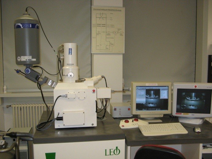
Fig. 14: SEM/EDS, Laboratory of Analytical Chemistry, Empa.
The analyses of slag inclusion in Fe-C alloys allow
inferences to be made regarding production techniques and the provenance of the
metal. This is, for example, shown in the study by Buchwald and Wivel 1998[24] in Scandinavia. In this
study the authors could show different provenance regions for the Fe studied
and the quality of the different manufacturing techniques used for Fe and
steel. They do not say how many analyses they performed per sample. Examples
show that they are numerous (in Table 1, Buchwald and Wivel 199810,
p77, nine analyses per sample are given). Dillmann and L’Héritier 2007[25] suggest some improvements
in the study of slag inclusions with SEM/EDS. They carried out about 40
analyses per sample. The analysing time was partly extended to 300 seconds and
the acceleration voltage generally decreased to 15kV. For this study between 5
and 12 slag inclusions are analysed at Empa per metal or metal strip.
Elemental analysis of corrosion products in the corrosion crust is not sufficient to determine their chemical formula and complementary structural analysis has to be carried out for this purpose. X-ray diffraction (XRD) analyses had been performed in the past on some samples (destructive analysis of particles). The results are included in the recorded sheets. Raman spectroscopy analysis is carried out on a restricted number of Cu corrosion products. XRD analysis is based on the diffraction of X-ray radiation by ordered materials like crystals, whereas Raman spectroscopy is based on the spectroscopic investigation of non-elastic scattering of light on crystals and other materials. Raman spectroscopy is carried out in a non-invasive way on the polished samples.
In Raman spectroscopy the difference in energy of oscillation condition between molecules and crystals is analysed. For this purpose a sample is illuminated by a laser light. The frequency (energy) of the monochromatic laser radiation is much higher than the differences in oscillation conditions of the molecules in the sample. Elastic Raleigh-scattering mostly occurs with only a limited proportion of emitted photons being generated by non-elastic scattering, known as Raman scattering. In this context oscillation of molecules or grid are excited by the laser. Light from the illuminated spot is collected with a lens and sent through a monochromator. Wavelengths close to the laser line (which are due to elastic Rayleigh scattering) are filtered out while the rest of the collected light is dispersed onto a detector. Spontaneous Raman scattering is typically very weak, and as a result the main difficulty of Raman spectroscopy is to separate the weak inelastically scattered light from the intense Rayleigh scattered laser light[26]. To identify Raman spectra references in publications, the web or personal records have been used.
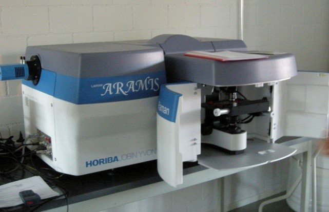
Fig. 15: Raman spectrometer, NMS, Affoltern am Ablis ZH.
The analyses are performed at the Conservation Laboratory of the Swiss National Museum at Affoltern a. Albis ZH with a LabRAM (Horiba Jobin Yvon) instrument coupled to three lasers with wavelength of 532nm, 633nm and 785nm (Fig. 15). To interpret the Raman spectra the composition and crystal structure of the standard materials are first measured as a control by WD-XRF and XRD. The same standard materials are analysed afterwards with Raman spectroscopy using different settings. The standard materials are: Cuprite/Cu2O: internal standard; Brochantite/CuSO4,3Cu(OH)2: internal standard; Chalcopyrite/CuFeS2: naturally occurring mineral in grain form (Alfa Aesar 42533); Covelline/CuS: internal standard and Tenorite/CuO: internal standard. In order to analyse them a laser with output at 532nm is used. The laser is directed into a microscope (magnification of x1000). The laser output power is 150mW, of which about 75 to 80mW reaches the sample when no filter is used. The different filters from D1 to D4 reduce the energy incident on the sample from 37 to 40mW to 0.0075mW. Before each sample is analysed a calibration with a Si-standard material is carried out. This calibration has to be done with 633nm laser.
The different settings are:
[1] Selwyn, L. (2004) Metals and corrosion: a handbook for the conservation professional. CCI, Ottawa.
[2] Scott, D. A. (1991) Metallography and microstructure of ancient and historic metals. The Getty Conservation Institute, Archetype Books, London.
[3] Bertholon, R. (2000) La limite de la surface d’origine des objets métalliques archéologiques – Caractérisation, localisation et approche des mécanismes de conservation, thèse de l’Université Paris I (https://tel.archives-ouvertes.fr/tel-00331190/document).
[4] Robbiola, L. and Hurtel, L. (1991) New contribution to the study of corrosion mechanisms of outdoor bronzes: characterization of the corroding surfaces of Rodin’s bronzes, Mémoires et Etudes Scientifiques Revue de métallurgie, 810-823 (https://hal.archives-ouvertes.fr/hal-00538986/document).
[5] Monnier, J. (2008) Corrosion atmosphérique sous abri d’alliages ferreux historiques. Caractérisation du système, mécanismes et apport à la modélisation, thèse de l’Université Paris-Est (https://tel.archives-ouvertes.fr/file/index/docid/374717/filename/These_Judith_Monnier.pdf).
[6] Garrels, R. M., and Christ, J.C. (1965) Solutions, minerals, and equilibria. San Francisco: Freeman, Cooper.
[7] Pourbaix M. (1963) Atlas d´équilibres électrochimiques à 25oC, Gauthier-Villars, Paris
[8] Pourbaix, M. (1977) Electrochemical corrosion and reduction, in Corrosion and Metal Artifacts. A dialogue Between Conservators and Archaeologists and Corrosion Scientists (B.F. Brown, H.C: Burnett, W.Th Chase, M. Goodway, J. Kruger, M. Pourbaix eds) NBS special publication 479, Washington, US Department of Commerce, National Bureau of Standards, 1-16.
[9] Robbiola, L. (1990) Caractérisation de l’altération de bronzes archéologiques enfouis à partir d’un corpus d’objets de l’Âge du bronze. Mécanismes de corrosion, these de l’Université Paris VI.
[10] Schweizer, F. (1994) Objets en bronze venant de sites lacustres : de leur patine à leur biographie, in L’œuvre d’art sous le regard des sciences, (éd. Rinuy, A. and Schweizer, F.), 143-157.
[11] Saheb, M., Neff, D., Dillmann, P. and Matthiesen, H. (2007) Long term corrosion behaviour of low carbon steel in anoxic soils, in METAL07, proceedings of the ICOM-CC Metal WG, Degrigny C, van der Lang R., Ankersmit B., Joosten I. (eds), Rijksmuseum, Amsterdam, 2, 69-75.
[12] Dillmann, P. (2004) Corrosion des objets archéologiques ferreux, Techniques de l’Ingénieur, COR 675, 1-20.
[13] Scott, D. A. (1991) Metallography and microstructure of ancient and historic metals. The Getty Conservation Institute, Archetype Books, London.
[14] Schumann, H. (1991) Metallographie. Leipzig.
[15] Stewart, J.W., Charles, J.A. and Wallach, E.R. (2000a) Iron-phosphorus-carbon system. Part 2 – Metallographic behaviour of Oberhoffer’s reagent. Materials Science and Technology, 16, 283-290.
[16] Stewart, J.W., Charles, J.A. and Wallach, E.R. (2000b) Iron-phosphorus-carbon system. Part 3 – Metallography of low carbon-phosphorus alloys. Materials Science and Technology, 16, 291-303.
[17] Devos, W., Senn-Luder, M., Moor, Ch., Salter, Ch. (2000) Laser ablation inductively coupled plasma mass spectrometry (LA-ICP-MS) for Spatially resolved trace analysis of early-medieval iron finds. Fresenius, Journal of Analytical Chemistry, 366, 873-880.
[18] Electron Microprobe, Wikipedia, accessed on April, 06, 2015.
[19] Northover, P. (1998) Analysis of copper alloy metalwork from Arbedo TI. In: Schindler, M.P. Der Depotfund von Arbedo TI. Antiqua 30, Basel. 289-315.
[20] Northover, J.P. (1985) The complete examination of archaeological metalwork. In Patricia Phillips et al. (ed.) The Archaeologist and the Laboratory, CBA Research Report 58, Council for British Archaeology, London.
[21] Inductively coupled plasma atomic emission spectroscopy, Wikipedia, accessed April, 06, 2015.
[22] Kläntschi, N. (1995) Die ICP-Analysen an der Empa. In: Rychner, V. and Kläntschi, N. Arsenic, nickel et antimoine. Cahier d’archéologie romande, 63, Lausanne, 14-16.
[23] Kronz, A. (1997). Phasenbeziehungen und Kristallisationsmechanismen in fayalitischen Schmelzsystemen – Untersuchungen an Eisen- und Buntmetallschlacken. Dissertation, Mainz.
[24] Buchwald, V.F. and Wivel, H. (1998) Slag analysis as a method for the characterisation and provenancing of ancient iron objects. Materials Characterization, 40, 73-96.
[25] Dillmann, P. and Héritier, M. (2007) Slag inclusions analyses for studying ferrous alloys employed in French medieval buildings: supply of materials and diffusion of smelting processes. Journal of Archaeological Science, 34, 1810-1823.
[26] Raman spectroscopy, Wikipedia, April, 06, 2015.